Udacity DLFND Project 1 Notes
Sat 25 March 2017 by Adrian TorrieThis post is part 1 of the "Udacity - Deep Learning Foundations Nanodegree" series:
Summary
Notes taken to help for the first project for the Deep Learning Foundations Nanodegree course dellivered by Udacity.
My Github repo for this project can be found here: adriantorrie/udacity_dlfnd_project_1
Table of Contents
Version Control
%run ../../../code/version_check.py
Change Log
Date Created: 2017-02-06

Date of Change    Change Notes
--------------    ----------------------------------------------------------------
2017-02-06        Initial draft
2017-03-23        Formatting changes for online publishing
Setup
%matplotlib inline

import matplotlib
import matplotlib.pyplot as plt
import numpy as np
import tensorflow as tf

plt.style.use('bmh')
matplotlib.rcParams['figure.figsize'] = (15, 4)
Neural network
Output Formula
Synonym
- The predicted value
- The prediction
Intuition
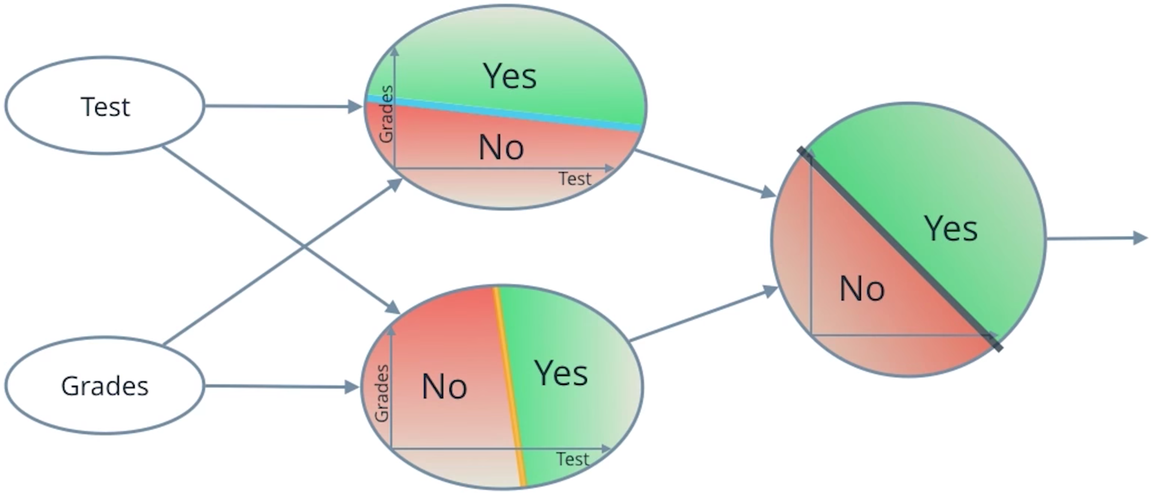
AND / OR perceptron
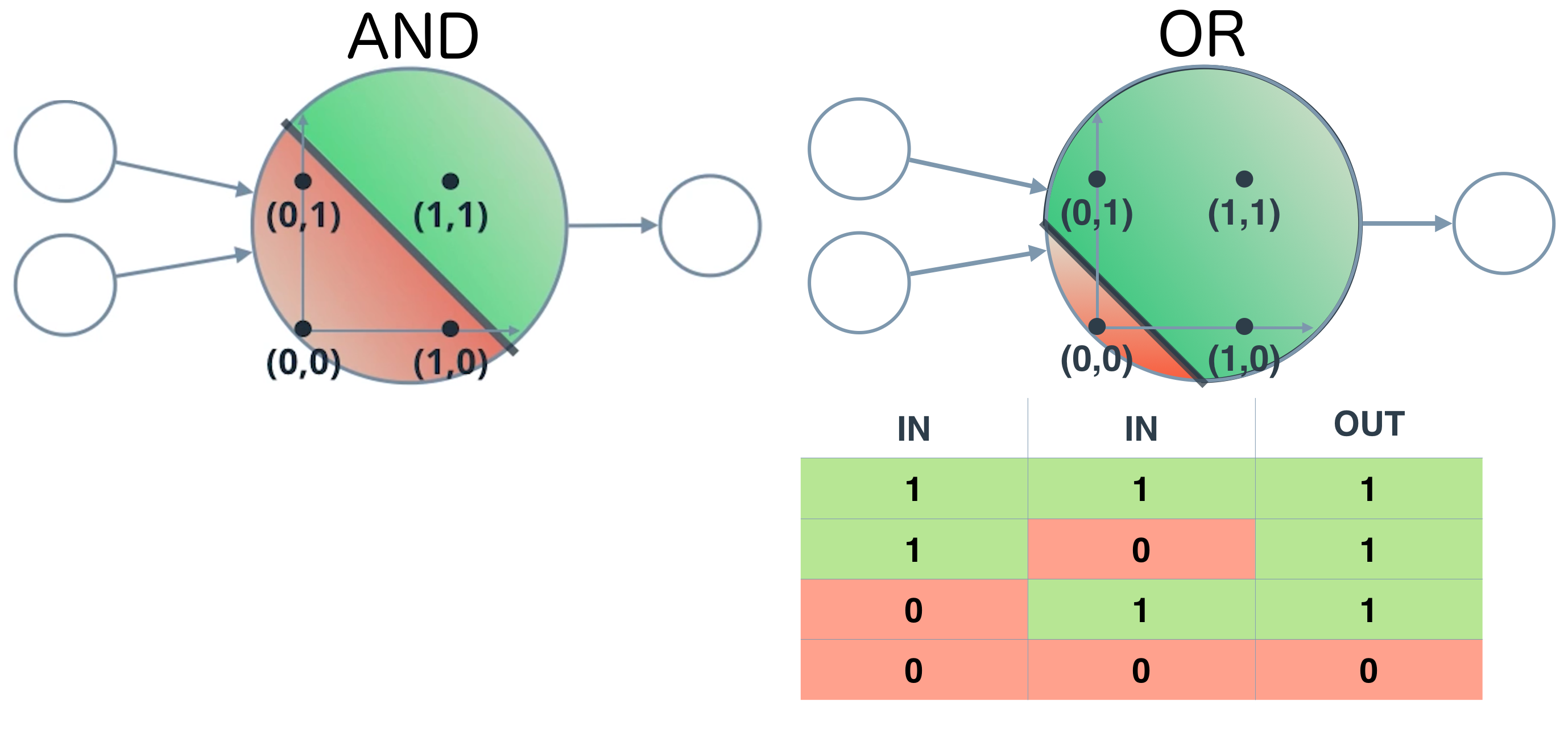
NOT perceptron
The NOT operations only cares about one input. The other inputs to the perceptron are ignored.
XOR perceptron
An XOR perceptron is a logic gate that outputs 0 if the inputs are the same and 1 if the inputs are different.
AF Summary
Activation functions can be for
- Binary outcomes (2 classes, e.g {True, False})
- Multiclass outcomes
Binary activation functions include:
- Sigmoid
- Hyperbolic tangent (and the alternative formula provided by LeCun et el, 1998)
- Rectified linear unit
Multi-class activation functions include:
- Softmax
Taken from Deep Learning Book - Chapter 6: Deep Feedforward Networks:
6.2.2 Output Units
- Any kind of neural network unit that may be used as an output can also be used as a hidden unit.
6.3 Hidden Units
- Rectified linear units are an excellent default choice of hidden unit. (My note: They are not covered in week one)
6.3.1 Rectified Linear Units and Their Generalizations
- g(z) = max{0, z}
- One drawback to rectified linear units is that they cannot learn via gradient-based methods on examples for which their activation is zero.
- Maxout units generalize rectified linear units further.
- Maxout units can thus be seen as learning the activation function itself rather than just the relationship between units.
- Maxout units typically need more regularization than rectified linear units. They can work well without regularization if the training set is large and the number of pieces per unit is kept low.
- Rectified linear units and all of these generalizations of them are based on the principle that models are easier to optimize if their behavior is closer to linear.
6.3.2 Logistic Sigmoid and Hyperbolic Tangent
- ... use as hidden units in feedforward networks is now discouraged.
- Sigmoidal activation functions are more common in settings other than feed-forward networks. Recurrent networks, many probabilistic models, and some auto-encoders have additional requirements that rule out the use of piecewise linear activation functions and make sigmoidal units more appealing despite the drawbacks of saturation.
- Note: Saturation as an issue is also in the extra reading, Yes, you should understand backprop, and also raised in Effecient Backprop, LeCun et el., 1998 and was one of the reasons cited for modifying the tanh function in this notebook.
6.6 Historical notes
- The core ideas behind modern feedforward networks have not changed substantially since the 1980s. The same back-propagation algorithm and the same approaches to gradient descent are still in use
- Most of the improvement in neural network performance from 1986 to 2015 can be attributed to two factors.
- larger datasets have reduced the degree to which statistical generalization is a challenge for neural networks
- neural networks have become much larger, due to more powerful computers, and better software infrastructure
- However, a small number of algorithmic changes have improved the performance of neural networks
- ... replacement of mean squared error with the cross-entropy family of loss functions. Cross-entropy losses greatly improved the performance of models with sigmoid and softmax outputs, which had previously suffered from saturation and slow learning when using the mean squared error loss
- ... replacement of sigmoid hidden units with piecewise linear hidden units, such as rectified linear units
Activation Formula
\begin{equation*} a = f(x) = \{sigmoid, tanh, softmax, \text{or some other function not listed in this set}\} \end{equation*}where:
- $a$ is the activation function transformation of the output from $h$, e.g. apply the sigmoid function to $h$
and
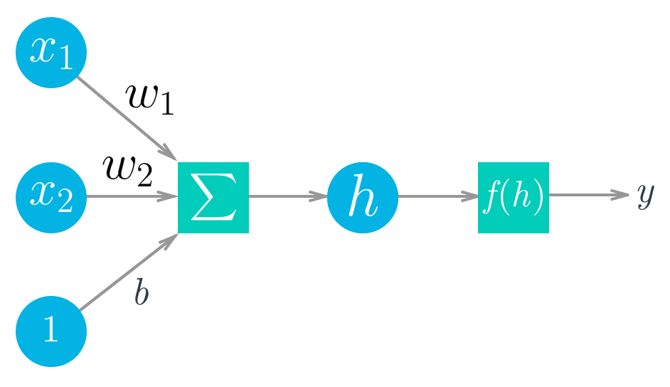
\begin{equation*} h = \Sigma_i w_i x_i + b \end{equation*}where:
- $x_i$ are the incoming inputs. A perceptron can have one or more inputs.
- $w_i$ are the weights being assigned to the respective incoming inputs
- $b$ is a bias term
- $h$ is the sum of the weighted input values + a bias figure
Sigmoid
Synonyms:
Summary
A sigmoid function is a mathematical function having an "S" shaped curve (sigmoid curve). Often, sigmoid function refers to the special case of the logistic function.
The sigmoid function is bounded between 0 and 1, and as an output can be interpreted as a probability for success.
Formula
\begin{equation*} \text{sigmoid}(x) = \frac{1} {1 + e^{-x}} \end{equation*}\begin{equation*} \text{logistic}(x) = \frac{L} {1 + e^{-k(x - x_0)}} \end{equation*}where:
- $L$ = the curve's maximum value
- $e$ = the natural logarithm base (also known as Euler's number)
- $x_0$ = the x-value of the sigmoid's midpoint
- $k$ = the steepness of the curve
Network output from activation
\begin{equation*} \text{output} = a = f(h) = \text{sigmoid}(\Sigma_i w_i x_i + b) \end{equation*}Code
def sigmoid(x):
    s = 1 / (1 + np.exp(-x))
    return s
inputs = np.array([2.1, 1.5,])
weights = np.array([0.2, 0.5,])
bias = -0.2

output = sigmoid(np.dot(weights, inputs) + bias)
print(output)
x = np.linspace(start=-10, stop=11, num=100)
y = sigmoid(x)

upper_bound = np.repeat([1.0,], len(x))
success_threshold = np.repeat([0.5,], len(x))
lower_bound = np.repeat([0.0,], len(x))

plt.plot(
    # upper bound
    x, upper_bound, 'w--',

    # success threshold
    x, success_threshold, 'w--',

    # lower bound
    x, lower_bound, 'w--',

    # sigmoid
    x, y
)

plt.grid(False)
plt.xlabel(r'$x$')
plt.ylabel(r'Probability of success')
plt.title('Sigmoid Function Example')
plt.show()

Tanh
Synonyms:
Summary
Just as the points (cos t, sin t) form a circle with a unit radius, the points (cosh t, sinh t) form the right half of the equilateral hyperbola.
The tanh function is bounded between -1 and 1, and as an output can be interpreted as a probability for success, where the output value:
- 1 = 100%
- 0 = 50%
- -1 = 0%
The tanh function creates stronger gradients around zero, and therefore the derivatives are higher than the sigmoid function. Why this is important can apparently be found in Effecient Backprop by LeCun et al (1998). Also see this answer on Cross-Validated for a representation of the derivative values.
Formula
\begin{equation*} \text{tanh}(x) = \frac{2} {1 + e^{-2x}} - 1 \end{equation*}\begin{equation*} \text{tanh}(x) = \frac{\text{sinh}(x)} {\text{cosh}(x)} \end{equation*}where:
- $e$ = the natural logarithm base (also known as Euler's number)
- $sinh$ is the hyperbolic sine
- $cosh$ is the hyperbolic cosine
Tanh Alternative Formula
\begin{equation*} \text{modified tanh}(x) = \text{1.7159 tanh } \left(\frac{2}{3}x\right) \end{equation*}Network output from activation
\begin{equation*} \text{output} = a = f(h) = \text{tanh}(\Sigma_i w_i x_i + b) \end{equation*}Code
inputs = np.array([2.1, 1.5,])
weights = np.array([0.2, 0.5,])
bias = -0.2

output = np.tanh(np.dot(weights, inputs) + bias)
print(output)
Example
x = np.linspace(start=-10, stop=11, num=100)
y = np.tanh(x)

upper_bound = np.repeat([1.0,], len(x))
success_threshold = np.repeat([0.0,], len(x))
lower_bound = np.repeat([-1.0,], len(x))

plt.plot(
    # upper bound
    x, upper_bound, 'w--',

    # success threshold
    x, success_threshold, 'w--',

    # lower bound
    x, lower_bound, 'w--',

    # sigmoid
    x, y
)

plt.grid(False)
plt.xlabel(r'$x$')
plt.ylabel(r'Probability of success (0.00 = 50%)')
plt.title('Tanh Function Example')
plt.show()

Alternative Example
def modified_tanh(x):
    return 1.7159 * np.tanh((2 / 3) * x)

x = np.linspace(start=-10, stop=11, num=100)
y = modified_tanh(x)

upper_bound = np.repeat([1.75,], len(x))
success_threshold = np.repeat([0.0,], len(x))
lower_bound = np.repeat([-1.75,], len(x))

plt.plot(
    # upper bound
    x, upper_bound, 'w--',

    # success threshold
    x, success_threshold, 'w--',

    # lower bound
    x, lower_bound, 'w--',

    # sigmoid
    x, y
)

plt.grid(False)
plt.xlabel(r'$x$')
plt.ylabel(r'Probability of success (0.00 = 50%)')
plt.title('Alternative Tanh Function Example')
plt.show()

Softmax
Synonyms:
Summary
Softmax regression is interested in multi-class classification (as opposed to only binary classification when using the sigmoid and tanh functions), and so the label $y$ can take on $K$ different values, rather than only two.
Is often used as the output layer in multilayer perceptrons to allow non-linear relationships to be learnt for multiclass problems.
Formula
From Deep Learning Book - Chapter 4: Numerical Computation
\begin{equation*} \text{softmax}(x)_i = \frac{\text{exp}(x_i)} {\sum_{j=1}^n \text{exp}(x_j)} \end{equation*}Network output from activation (incomplete)
\begin{equation*} \text{output} = a = f(h) = \text{softmax}() \end{equation*}Code
Link for a good discussion on SO regarding Python implementation of this function, from which the code below code was taken from.
def softmax(X):
    assert len(X.shape) == 2
    s = np.max(X, axis=1)
    s = s[:, np.newaxis] # necessary step to do broadcasting
    e_x = np.exp(X - s)
    div = np.sum(e_x, axis=1)
    div = div[:, np.newaxis] # dito
    return e_x / div

X = np.array([[1, 2, 3, 6],
              [2, 4, 5, 6],
              [3, 8, 7, 6]])
y = softmax(X)
y
# compared to tensorflow implementation
batch = np.asarray([[1,2,3,6], [2,4,5,6], [3, 8, 7, 6]])
x = tf.placeholder(tf.float32, shape=[None, 4])
y = tf.nn.softmax(x)

init = tf.global_variables_initializer()
sess = tf.Session()

sess.run(y, feed_dict={x: batch})
Gradient Descent
Learning weights
What if you want to perform an operation, such as predicting college admission, but don't know the correct weights? You'll need to learn the weights from example data, then use those weights to make the predictions.
We need a metric of how wrong the predictions are, the error.
Sum of squared errors (SSE)
\begin{equation*} E = \frac{1}{2} \Sigma_u \Sigma_j \left [ y_j ^ \mu - \hat y_j^ \mu \right ] ^ 2 \end{equation*}where (neural network prediction):
\begin{equation*} \hat y_j^\mu = f \left(\Sigma_i w_{ij} x_i^\mu\right) \end{equation*}therefore:
\begin{equation*} E = \frac{1}{2} \Sigma_u \Sigma_j \left [ y_j ^ \mu - f \left(\Sigma_i w_{ij} x_i^\mu\right) \right ] ^ 2 \end{equation*}Goal
Find weights $w_{ij}$ that minimize the squared error $E$.
How? Gradient descent.
Gradient Descent Formula
\begin{equation*} \Delta w_{ij} = \eta (y_j - \hat y_j) f^\prime (h_j) x_i \end{equation*}remembering $h_j$ is the input to the output unit $j$: \begin{equation} h = \sumi w{ij} x_i \end{equation}
where:
- $(y_j - \hat y_j)$ is the prediction error.
- The larger this error is, the larger the gradient descent step should be.
- $f^\prime (h_j)$ is the gradient
- If the gradient is small, then a change in the unit input $h_j$ will have a small effect on the error.
- This term produces larger gradient descent steps for units that have larger gradients
The errors can be rewritten as: \begin{equation} \delta_j = (y_j - \hat y_j) f^\prime (h_j) \end{equation}
Giving the gradient step as: \begin{equation} \Delta w_{ij} = \eta \delta_j x_i \end{equation}
where:
- $\Delta w_{ij}$ is the (delta) change to the $i$th $j$th weight
- $\eta$ (eta) is the learning rate
- $\delta_j$ (delta j) is the prediction errors
- $x_i$ is the input
Algorithm
- Set the weight step to zero: $\Delta w_i = 0$
- For each record in the training data:
- Make a forward pass through the network, calculating the output $\hat y = f(\Sigma_i w_i x_i)$
- Calculate the error gradient in the output unit, $\delta = (y − \hat y) f^\prime(\Sigma_i w_i x_i)$
- Update the weight step $\Delta w_i= \Delta w_i + \delta x_i$
- Update the weights $w_i = w_i + \frac{\eta \Delta w_i} {m}$ where:
- η is the learning rate
- $m$ is the number of records
- Here we're averaging the weight steps to help reduce any large variations in the training data.
- Repeat for $e$ epochs.
Code
# Defining the sigmoid function for activations
def sigmoid(x):
    return 1 / ( 1 + np.exp(-x))

# Derivative of the sigmoid function
def sigmoid_prime(x):
    return sigmoid(x) * (1 - sigmoid(x))

x = np.array([0.1, 0.3])
y = 0.2
weights = np.array([-0.8, 0.5])
# probably use a vector named "w" instead of a name like this
# to make code look more like algebra

# The learning rate, eta in the weight step equation
learnrate = 0.5

# The neural network output
nn_output = sigmoid(x[0] * weights[0] + x[1] * weights[1])
# or nn_output = sigmoid(np.dot(weights, x))

# output error
error = y - nn_output

# error gradient
error_gradient = error * sigmoid_prime(np.dot(x, weights))
# sigmoid_prime(x) is equal to -> nn_output * (1 - nn_output)

# Gradient descent step
del_w = [ learnrate * error_gradient * x[0],
          learnrate * error_gradient * x[1]]
# or del_w = learnrate * error_gradient * x
Caveat
Gradient descent is reliant on beginnning weight values. If incorrect could result in convergergance occuring in a local minima, not a global minima. Random weights can be used.
Momentum Term
The momentum term increases for dimensions whose gradients point in the same directions and reduces updates for dimensions whose gradients change directions. As a result, we gain faster convergence and reduced oscillation.
Multilayer Perceptrons
Synonyms
- MLP (just an acronym)
Numpy column vector
Numpy arays are row vectors by default, and the input_features.T (transpose) transform still leaves it as a row vector. Instead we have to use (use this one, makes more sense):
input_features = input_features[:, None]
Alternatively you can create an array with two dimensions then transpose it:
input_features = np.array(input_features ndim=2).TCode example setting up a MLP
# network size is a 4x3x2 network
n_input = 4
n_hidden = 3
n_output = 2

# make some fake data
np.random.seed(42)
x = np.random.randn(4)

weights_in_hidden = np.random.normal(0, scale=0.1, size=(n_input, n_hidden))
weights_hidden_out = np.random.normal(0, scale=0.1, size=(n_hidden, n_output))

print('x shape\t\t\t= {}'.format(x.shape))
print('weights_in_hidden shape\t= {}'.format(weights_in_hidden.shape))
print('weights_hidden_out\t= {}'.format(weights_hidden_out.shape))
Backpropogation
When doing the feed forward pass we are taking the inputs and using the weights (which are randomly assigned) to gain an output. In backprop you can view this as the errors (difference between prediction and actual expected value) being passed through the network using the weights again.
Worked example
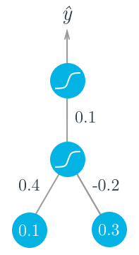
- Two layer network (Inputs not considered a layer, 1 hidden layer, 1 output layer):
- Assume target outcome is $y = 1$.
- Forward pass:
- Sigmoid input = $h = \Sigma_i w_i x_i = 0.1 \times 0.4 - 0.2 \times 0.3 = -0.02$
- Activtion function = $a = f(h) = \text{sigmoid}(-0.02) = 0.495$
- Predicted output = $ \hat y = f(W \cdot a) = \text{sigmoid}(0.1 \times 0.495) = 0.512$
- Backwards pass:
- Sigmoid derivate = $f^\prime (W \cdot a) = f(W \cdot a)(1 - f(W \cdot a))$
- Output error = $\delta^o = (y - \hat y)f^\prime(W \cdot a) = (1 - 0.512) \times 0.512 \times (1 - 0.512) = 0.122$
- Usual hidden units error = $\delta_j^h = \Sigma_k W_{jk} \delta_k^o f^\prime(h_j)$
- This example single hidden unit error = $\delta^h = W \delta^o f^\prime(h) = 0.1 \times 0.122 \times 0.495 \times (1 - 0.495) = 0.003$
- Gradient descent step (output to hidden) = $\Delta W = \eta \delta^o a = 0.5 \times 0.122 \times 0.495 = 0.0302$
- Gradient descent step (hidden to inputs) = $\Delta w_i = \eta \delta^h x_i = (0.5 \times 0.003 \times 0.1, 0.5 \times 0.003 \times 0.3) = (0.00015, 0.00045)$
From this example, you can see one of the effects of using the sigmoid function for the activations. The maximum derivative of the sigmoid function is 0.5, so the errors in the output layer get scaled by at least half, and errors in the hidden layer are scaled down by at least a quarter. You can see that if you have a lot of layers, using a sigmoid activation function will quickly reduce the weight steps to tiny values in layers near the input.
Backprop algorithm for updating the weights
- Set the weight steps for each layer to zero
- The input to hidden weights $\Delta w_{ij} = 0$
- The hidden to output weights $\Delta W_j = 0$
- For each record in the training data:
- Make a forward pass through the network, calculating the output $\hat y$
- Calculate the error gradient in the output unit, $\delta^o = (y − \hat y)f^\prime(z)$
- Where the input to the output unit = $z = \Sigma_j W_j a_j$,
- Propagate the errors to the hidden layer $\delta_j^h = \delta^o W_j f^\prime(h_j)$
- Update the weight steps:
- $\Delta W_j = \Delta W_j + \delta^o a_j$
- $\Delta w_{ij} = \Delta w_{ij} + \delta_j^h a_i$
- Update the weights, where $\eta$ is the learning rate and $m$ is the number of records:
- $W_j = W_j + \frac {\eta \Delta W_j} {m}$
- $w_{ij} = w_{ij} + \frac {\eta \Delta w_{ij}} {m}$
- Repeat for $e$ epochs.
Additional Reading
- Understanding the backward pass through Batch Normalization Layer
- Yes, you should understand backprop
- Effecient Backprop, LeCun et el., 1998
- Good intuition of momentum term in gradient descent
- Deep Learning Book - Chapter 4: Numerical Computation
- Deep Learning Book - Chapter 6: Deep Feedforward Networks
